10. Additional components
Gamman can be expanded with components or "tools" for specific purposes.
The "tools" presently available are
- Background editor
- Coordinate conversion
- Aux data import
- Airborne corrections
- Calibration toolbox
- Borehole corrections
- Scripter
Airborne corrections
Gamman has extensive options for the correction of airborne data. Two options are available for processing the raw data, a 'classic' process option and an option based on the full spectrum analysis. These processing options also contain several parameters to improve the quality of the data. One can for example compensate for radiation originating from the plane, use radon calibration data and apply height corrections.
"Classic" correction of airborne data is implemented according to the guidelines of the IAEA (IAEA TECDOC- 1363). It involves correction of airborne radiometric data by using a standard elevation-dependent absorption model and an effective height based on pressure and air temperature. It also allows to include a radon background and plane background for subtraction from the measured data.
"FSA-based" correction of airborne data is an entirely different approach to airborne corrections. The model is based on using elevation dependent full spectrum analysis. That is, GAMMAN contains a library of calibration spectra for each elevation between 0.5 and 160m elevation for 4x4x16 NaI and CsI systems/packs and spectra for elevations between 0 and 40m elevation for MS2000 and smaller detectors. For each elevation, a set of standard spectra was created that incorporates the effects of (energy-dependent) radiation absorption in air. It also includes a calibration or standard spectrum for Radon (Rn) in air.
The algorithm is as follows:
Estimate the radon contribution. This is done by fitting K, U, Th and Rn spectra to each spectrum as a function of elevation. Though originating from merely the same radiating nuclide (Bismuth), the Rn and U spectra are strongly different, especially at the low-energy sides of the spectra. The reason for this being the difference in absorption suffered by the Rn radiation (in air) and the U radiation (from the soil). The full spectrum algorithm will separate the Rn signal from the U signal because of this difference.
Use the Rn activity to estimate for each nuclide the background, and sum with the cosmic background (based on a cosmic spectrum scaled to the counts in the cosmic channel) and a plane background.
Substract background from each spectrum and fit with K, U and Th spectra for the elevation under consideration.
The FSA algorithm thus includes all airborne calibrations at once; without the need of using an upward looking detector for Rn estimation.
Classic
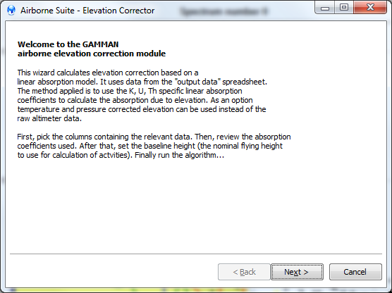
The "classic" airborne corrections wizard can be accessed at Tools | Classic elevation corrections…
The following pages are present in the "classic" airborne corrections wizard:
The welcome screen;
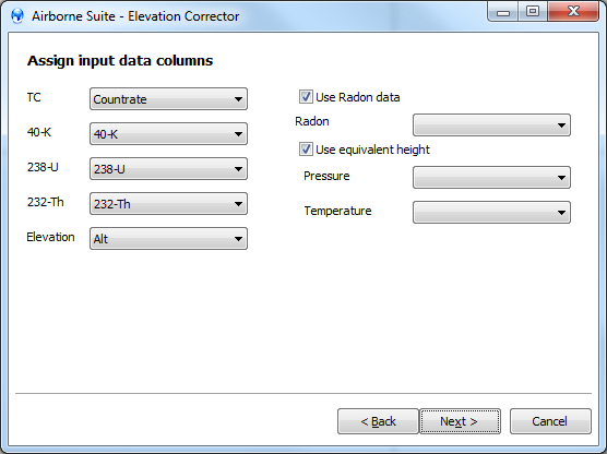
Assigning the input columns.
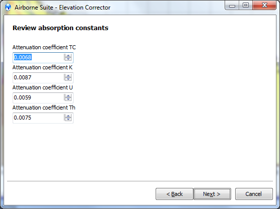
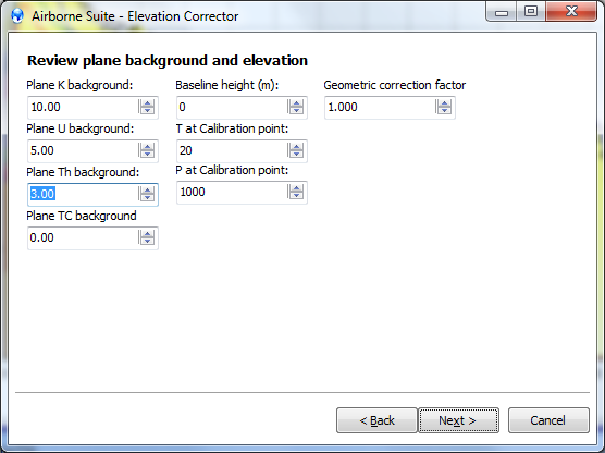
Setting the attenuation coefficients;
To set the plane background, baseline height (the baseline is the elevation that all nuclide concentrations are calculated to), and Temperature (T) and Pressure (P) at the calibration point for the P, T sensor used in the survey. A geometric correction factor can be used to scale all nuclide concentrations.
Full spectrum
The "Full Spectrum Analysis-based" airborne corrections wizard can be accessed at Spectral Analysis | Full-spectrum elevation correction
More information about the methodology can be found at Airborne corrections
The following pages are present in the "FSA-based" airborne corrections wizard:
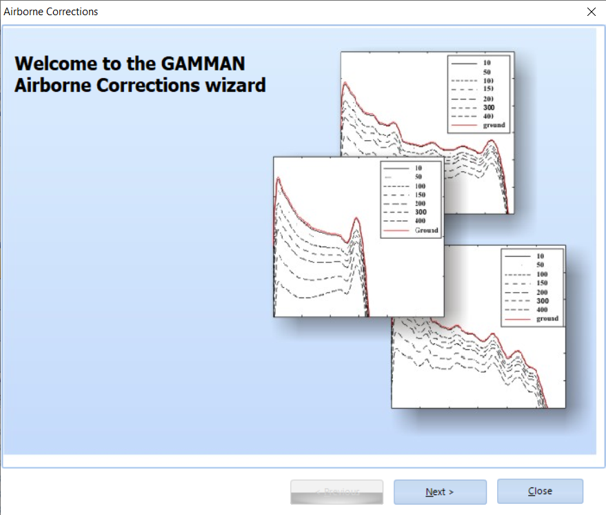
Page 1: welcome page
Page 2: settings for airborne processing.
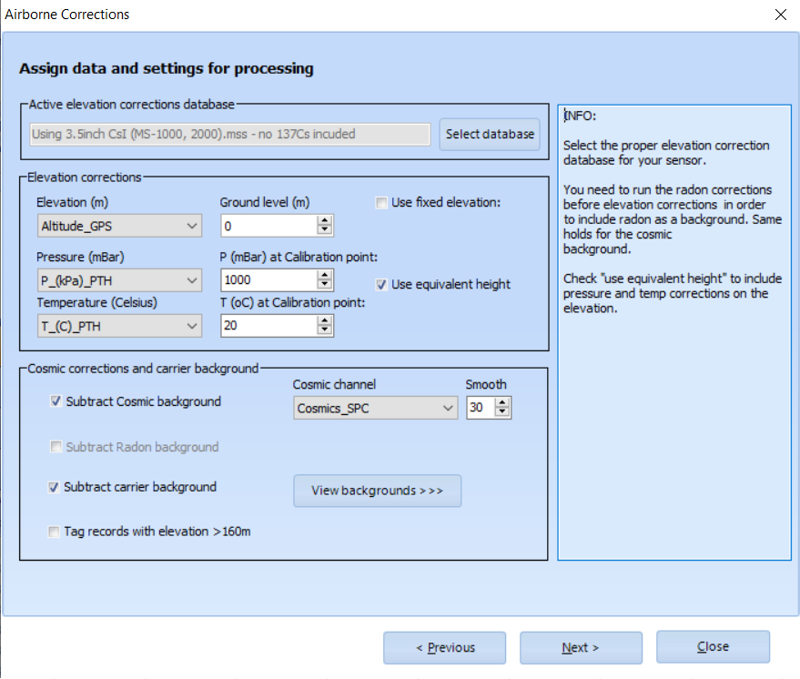
In Elevation corrections, the columns containing elevation, temperature and pressure data can be assigned. Checking the box Use fixed elevation will ignore the elevation column and instead applies the fixed elevation that is filled in.
In Radon corrections, one can choose to incorporate Rn. A scaler field is used to increase or decrease the amount of Rn that is subtracted (micro-leveling).
In Cosmic corrections and carrier background, the parameters for cosmic background can be set. When choosing to incorporate cosmic background, the channel containing the cosmic counts (i.e. counts above 3MeV) can be chosen in the box Cosmic channel. Also, it can be chosen how much to smooth the cosmic background. The knob View backgrounds opens a simple spectrum viewer showing the currently active carrier and cosmic backgrounds. The option to subtract the carrier background can be checked.
The option Tag records with elevation >160m will exclude all records that have an elevation beyond 160m.
The last page shows the processing of the data.
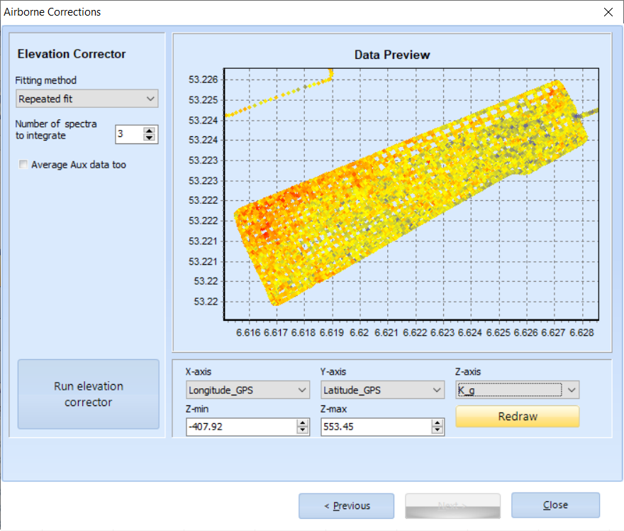
Here one can choose to sum a number of spectra for better fit-results using a smart fit or repeated fit method. Process the data by clicking the button Run elevation corrector. Results can be visualized in the plotter on this page. When happy with the height corrected results, save the processed data by clicking the close button. A dialog will appear where a name can be given to the new data tab that will be created.
After finishing processing the complete dataset, the new data tab window is present in the GAMMAN main screen and filled with the airborne FSA data just calculated.
Cosmic spectrum builder
The "Cosmics" airborne corrections can be accessed at Spectral Analysis | Cosmic spectrum builder…
More information about the methodology can be found at Cosmic and carrier backgrounds
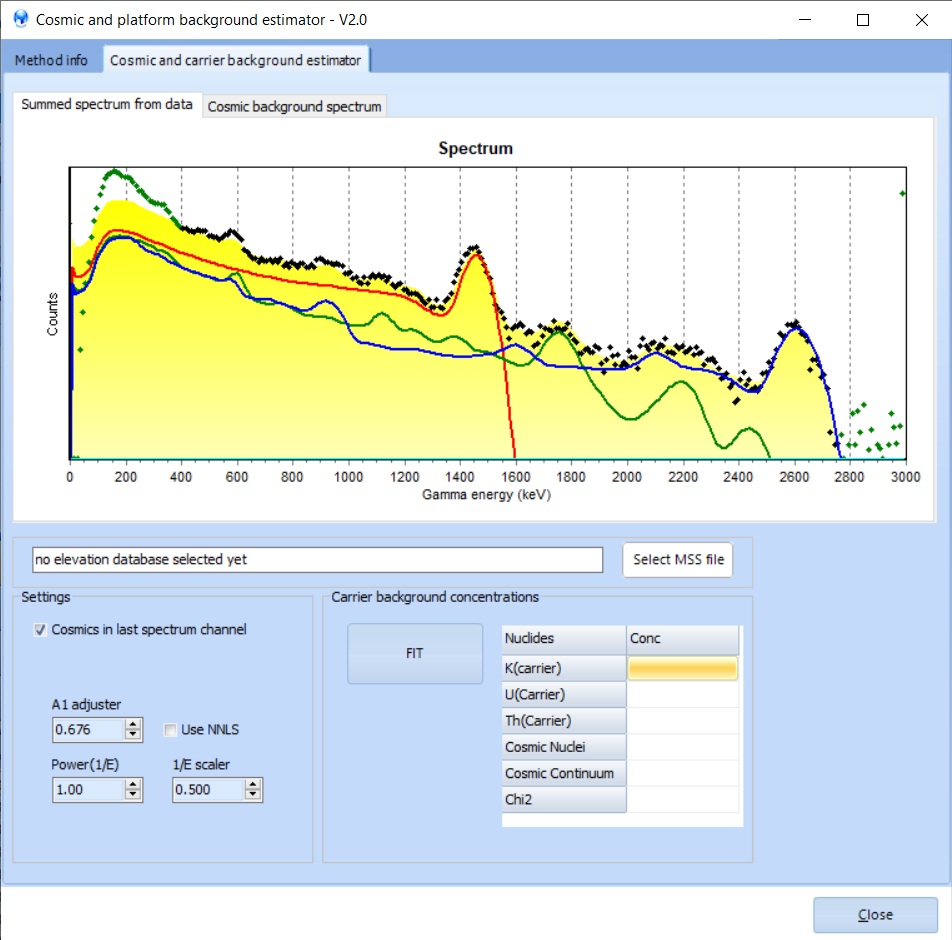
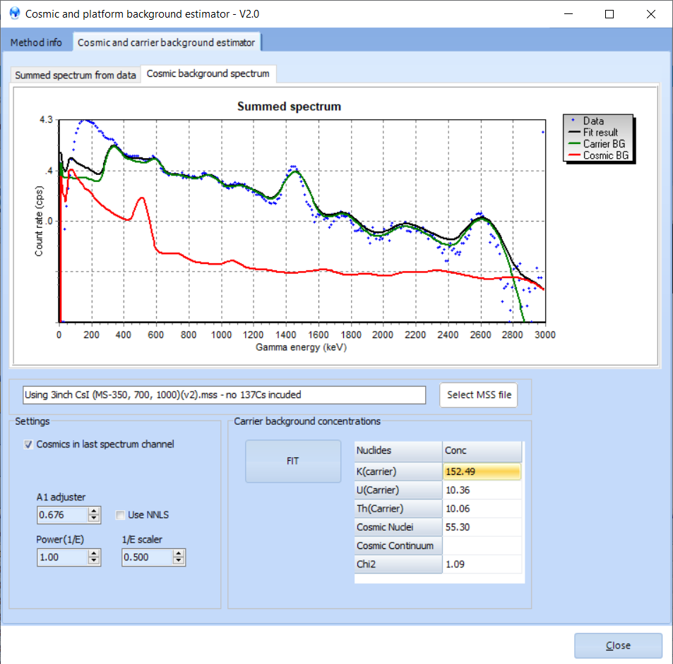
The Cosmic and carrier background estimator wizard starts with a page about the method info. The second page is the background estimator and consists of the following two tabs: the “Summed spectrum from data” and “Cosmic background spectrum”.
The first shows the complete summed spectrum from all the selected data records together with the standard spectra, the other shows the standard cosmic and carrier background spectra that needs to be fitted under the measured spectrum.
On both pages, fitting parameters can be adjusted. These are the mss-file, which holds a detector-type specific database with elevation dependent spectra, column cosmic counts and other spectrum shape settings. Pressing “Fit” incorporates these settings.
Save the backgrounds by pressing “Close”. They are then stored in the project file.
Classic cosmic background finder
This cosmic spectrum builder is based on guidelines according to the IAEA. It can be found by navigating to Tools | Classic cosmic background finder. The opening page of the cosmic spectrum builder shows the summed spectrum from the selection made before opening the wizard. In the box labeled "Cosmic Data" you can either pick the column in the input dataset that contains the cosmic counts, or choose the cosmics stored in the last spectrum channel. By clicking the Determine cosmic and carrier spectrum you start the deconvolution process that determines the background spectra. After finishing, the other TABs contain the resulting cosmic and carrier background spectra. By pressing the Smoothen button, the cosmic spectrum can be filtered by 5 point smoothening, allowing to remove statistical noise inherent to the cosmic data. After pressing Close you will be asked to store the spectra or discard them.
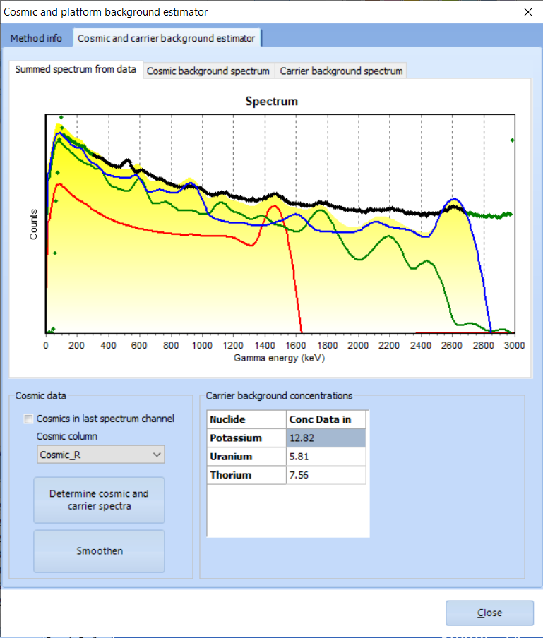
Summed spectrum of the selected data records
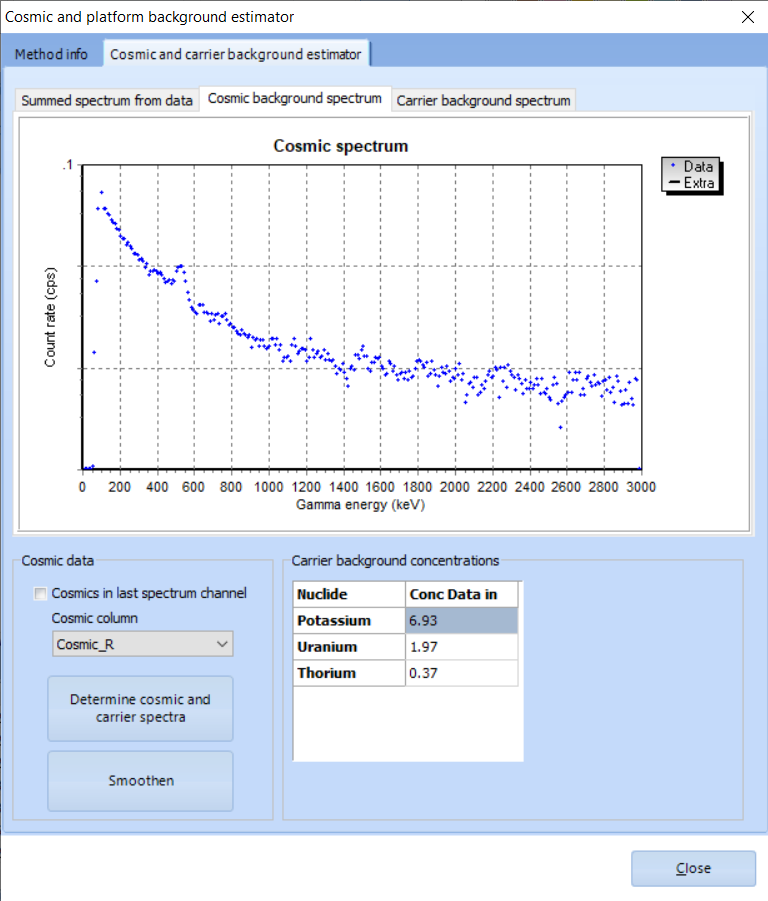
Determined (unsmoothened) cosmic background spectrum. Note the 511 keV annihilation peak.
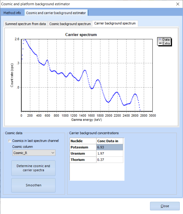
Determined carrier background spectrum. The table lists the actual activity concentrations found in the carrier background.
Background editor
Gamman supports three different backgrounds to be taken into account in the analysis of spectra:
1. A general background;
2. The "carrier" background;
3. The "cosmic" background.
The purpose and handling of these backgrounds deserves a bit of attention. The general background is the only background that can be used in the standard analysis part of Gamman. That is, whenever a spectrum is designated as a general background spectrum, it will be subtracted from the measured spectra before analysis. The carrier and cosmic background spectra are only used in the airborne corrections module, available as an additional component.
The background editor window (see below) provides a view on the background spectra currently active in your project. Calibration | Background editor
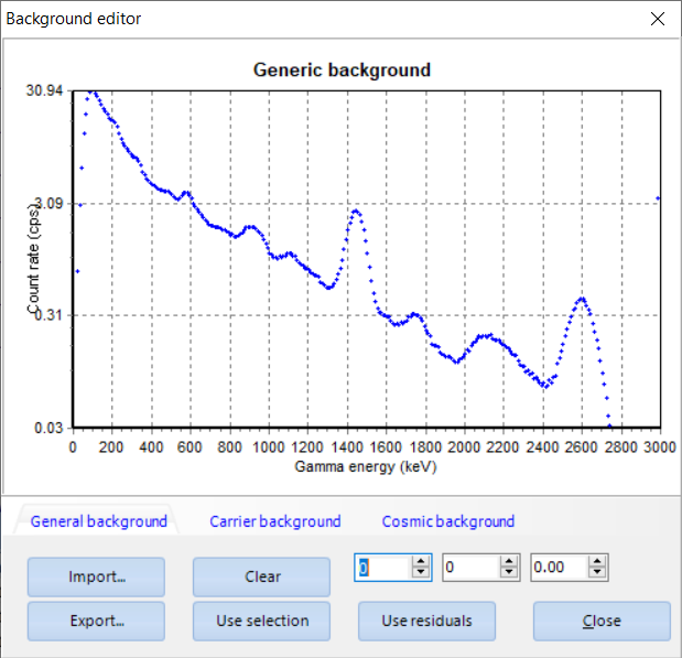
The three TABs allow to switch between general, carrier and cosmic backgrounds.
Item | Description |
|---|---|
Import | Open a spectrum file (an ASCII file containing 300 channel spectra) and use its data as a background spectrum. |
Export | Save the currently visible spectrum as a 300 channel ASCII spectrum. |
Clear | Clear the selected background spectrum |
Use selection (general background only) | Use the (summed) spectrum currently visible in the Gamman main window as a background spectrum from the data currently loaded. |
Use residuals |
Calibration
Gamman also supports viewing and editing the calibration data used in a project. The relevant tab in the menu [Calibration] has a few submenu's.
Edit active calibration
Via Calibration | Edit active calibration data you can open a form that displays the parameters set in the calibration data active in your project. Via Calibration | Edit calibration file] the same form is opened, displaying a user-selected calibration file.
CAUTION: Changing calibration parameters may hugely affect the results of the data analysis. Be precautious, especially when changing the calibration files without making a backup first. More information about calibration files can be found at Calibration files.
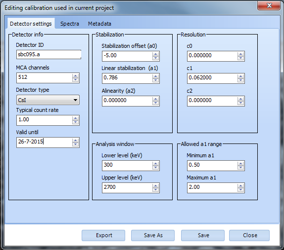
TAB 1 contains the "Detector settings", most of which cannot be changed. The detector's ID, the number of MCA channels it provides, the detector type and the typical count rate are displayed. Also listed is a date that determines the end of the validity of the sensor's calibration data. This is an indicative date only, mostly about five years ahead of the actual calibration date.
The stabilization parameters set for the instrument are listed in the "Stabilization" box. At the bottom you see the "Analysis window" (the range in keV of the spectrum that is used in the full spectrum analysis). The "Allowed a1 range" is used by the stabilization algorithm to see if the stabilization found is within reasonable limits. For more on stabilization, see Stabilization. The resolution of the system is listed in the "Resolution" box. The numbers here are used by the airborne correction wizard to construct spectra for each elevation flown in your survey.
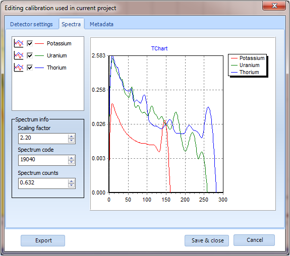
TAB two displays the spectra. By clicking a check, the spectrum will be hidden or displayed. The spectrum info block displays the scaling factor used for this spectrum, the spectrum code and the total count inside the spectrum. Remember, the spectra are defined as the response of your system to a source of 1 Bq/kg activity in a certain geometry and density.
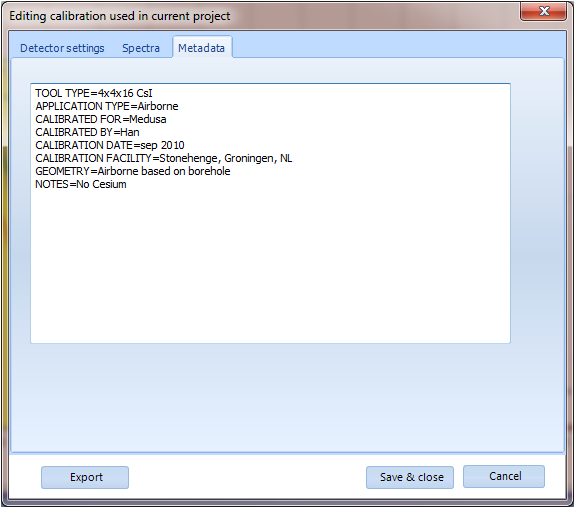
TAB 3 displays some meta-data relevant for the calibration data.
Edit calibration file
See edit active calibration
Replace calibration data
This option lets you select a calibration file (.mcf) which will replace the current calibration file. Be aware that this will clear the processed data already generated and might require a restabilization.
Re-run energy calibration
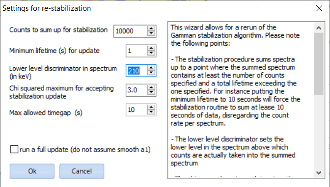
It is also possible to redo the stabilization process for the complete Gamman dataset. In the dialog box that appears, some parameters need to be filled in. The settings are explained in the text shown in this dialog box.
Aux data import
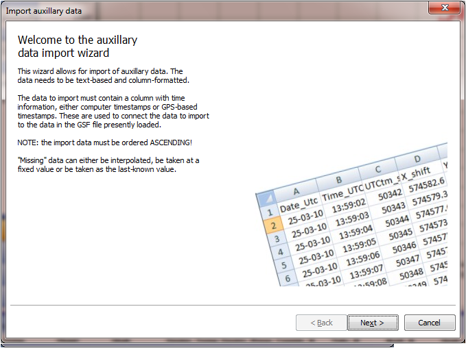
Sometimes, it is handy to be able to import auxiliary data. Such data may for instance contain measurements of other sensors during the same survey in which your radiometry data was taken. This could be other geophysical data (EM, magnetometry, etc) and/or data from elevation meters, GPS, temperature and pressure, etc. Gamman now supports merging this auxiliary data into your raw data spreadsheet. The auxiliary data needs to be formatted as a spreadsheet; it should be time-ordered and it should contain a "key" column that can be merged with a "key" column in the raw data. Mostly this will be a column containing some timestamp (GPS time for instance).
The following describes the pages of this wizard which can be accessed through File | Import aux data.
Page 1 displays a welcome screen.
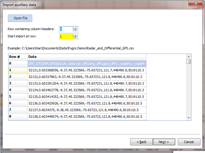
Page 2 allows to open and preview the file you want to import.
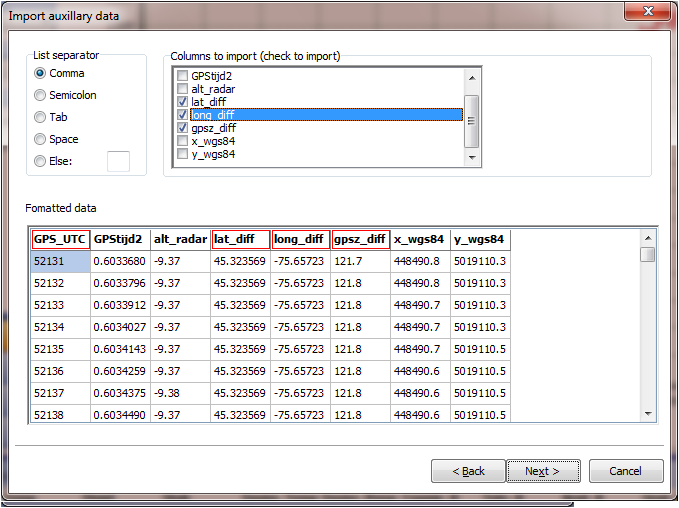
On page 3, you pick a column separator (most of the time, Gamman will find the separation for you). You can also pick the columns you want to have imported into your raw data.
Page 4 allows to do the actual merge of the data.
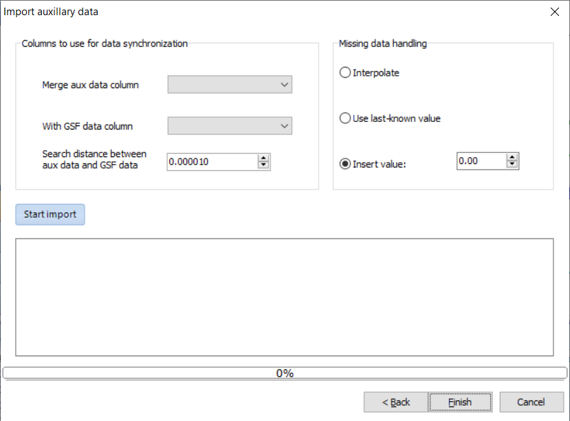
Select the column in the aux data that is used to match rows in the aux data sheet with the corresponding rows in the raw Gamman data. Normally these columns would contain time data of a clock known in both datasets. The edit box Search distance allows to search for the closest value in gsf data to a value in the auxiliary data merge column.
The "Missing data handling" box allows to select what to do if no matching record in the aux data is found for a certain row of raw data in your Gamman project. Either the data is constructed by interpolating between the two nearest rows that do contain data; or the last known value is used, or a value is inserted.
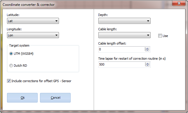
Coordinate conversion
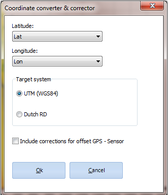
When the GPS is not positioned on top of the detector an offset can be applied to calculate the detector measurement location coordinates. In case of water-surveys, columns can be selected for depth and cable length. 'Cable length offset' is the offset between the position of the GPS and the start of the cable.
The coordinate converter can be found at Tools | coordinate conversion.
Borehole corrections
Borehole corrections
The borehole corrections wizard can be accessed at Tools | Borehole corrections
The 'Borehole correction' wizard enables the calculation of reference borehole data from measured borehole data. The geometry and composition of the borehole and the position of the detector influence the measurement. When the measured data is corrected, data from different boreholes can be compared and interpreted.
The corrections are applied on processed data.
Corrections that can be performed are corrections for:
· Borehole diameter
· Casing thickness
· Probe position
· Formation Density
· Fluid density
· Fluid activity
After the welcome screen, the properties of the measured borehole can be entered in the "Borehole properties" box shown below.
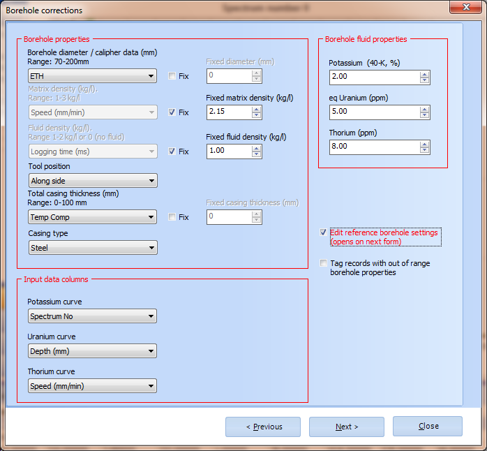
Either a column in which the data is listed can be selected or a fixed value can be entered in the box after checking the fix box. Properties of the borehole fluid can be entered in the box to the right, mind the units! The input data columns are the columns in the processed data that will be used for the correction. Two boxes to the lower right allow to edit the reference borehole settings or to tag records that are out of range and will be discarded form the calculation.
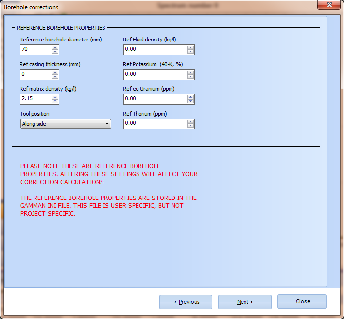
The third page of the wizard, shown above, only opens when the "edit reference borehole settings" checkbox is set (see 2nd wizard page). The reference borehole is the standard borehole configuration used as a baseline for all calculations. Please note that changing the reference values will affect the correction. After processing, the columns with corrected nuclide data will be added to the Processed data data view as a set of extra columns containing the corrected K, U, Th and TC values.
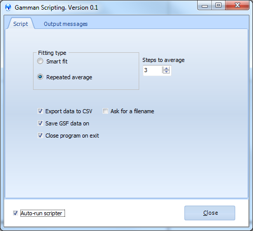
Scripter
The ´Scripter´ wizard can be accessed at Tools | Scripter This tool has been written to speed up or automate 'standard' Gamman analysis and processing. Only basic functionality has been included, any (airborne or other) corrections or checks cannot be performed using Scripter. Scripter facilitates two processing options, 'smart fit' and 'repeated average'. More information on the processing options can be found at Fitting schemes. Export, save project and close program options can be chosen. Data will be stored in de input data root. When the 'Ask for a filename' box is not checked the default filename is the filename of the first input file. Scripter can handle all possible input file types and performs a stabilization of the data first. When the box 'Auto-run scripter' is checked, Scripter will auto-run the above checked procedures after loading new input data. When checking Show Scripter warning in the Edit | Program settings window, a warning will pop-up at data import, reminding you that the Auto-run functionality of Scripter is enabled.