Application manual

This manual explains how to correctly use a Medusa gamma-ray spectrometer during field operations. It covers preparation, assembly, data acquisition, pausing, downloading, and data processing. Follow the steps carefully to ensure reliable and reproducible results.

Survey execution

Preparation

• Before a survey, make sure the power sources (power banks and batteries) are sufficient and full.

• Pack all the things you need and check that you have packed all necessary components:

  • Fully charged power banks/batteries

  • Backpack (for walking surveys)

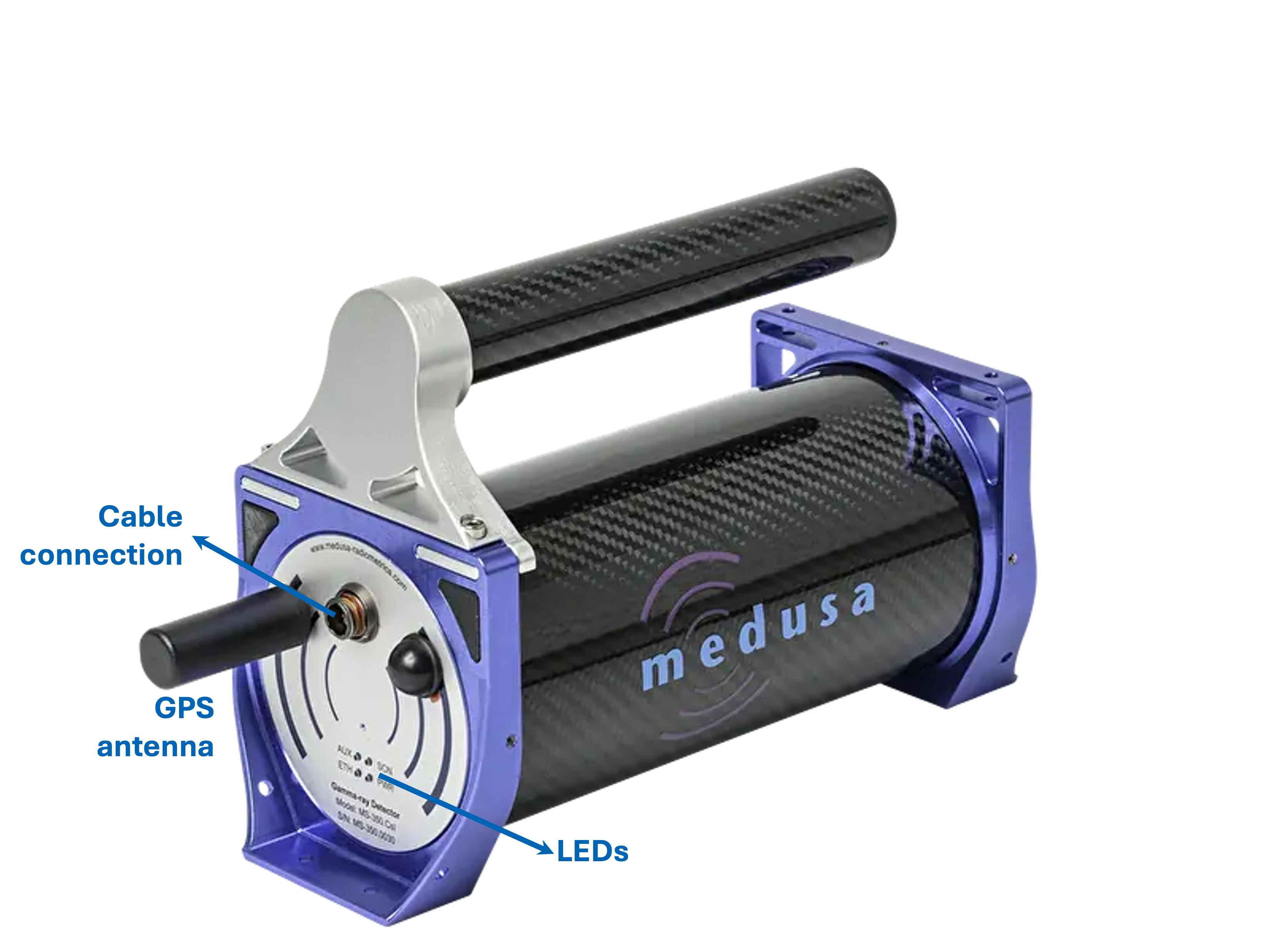
  • GPS antenna

  • Connection cables

  • Charged phone, tablet or laptop

Assembly On Site

• After transporting the instrument to the field in its protective case, assemble everything ready for use:

  • Attach the GPS antenna,

  • If applicable: place sensor on the backpack frame

  • switch the sensor on by connecting the power cable (It is best done at the survey starting point because the sensor starts to measure as soon as it gets the power.)

  • Connect the phone, tablet or PC.

Connecting to the detector

• After powering the sensor, you can connect to its Wi-Fi from your device. The name of the connection point is

  • Wifi Network name: MS-<model>-<serial> (e.g. MS-1000-0044),

  • Password: @Radiometrics123.

• Open a browser and go to the URL 192.168.3.1. If you have an android device, you can use the mDOS app. It shows the connected sensor; just click on it, and it brings you to the same address by opening your default browser.

Data quality checks

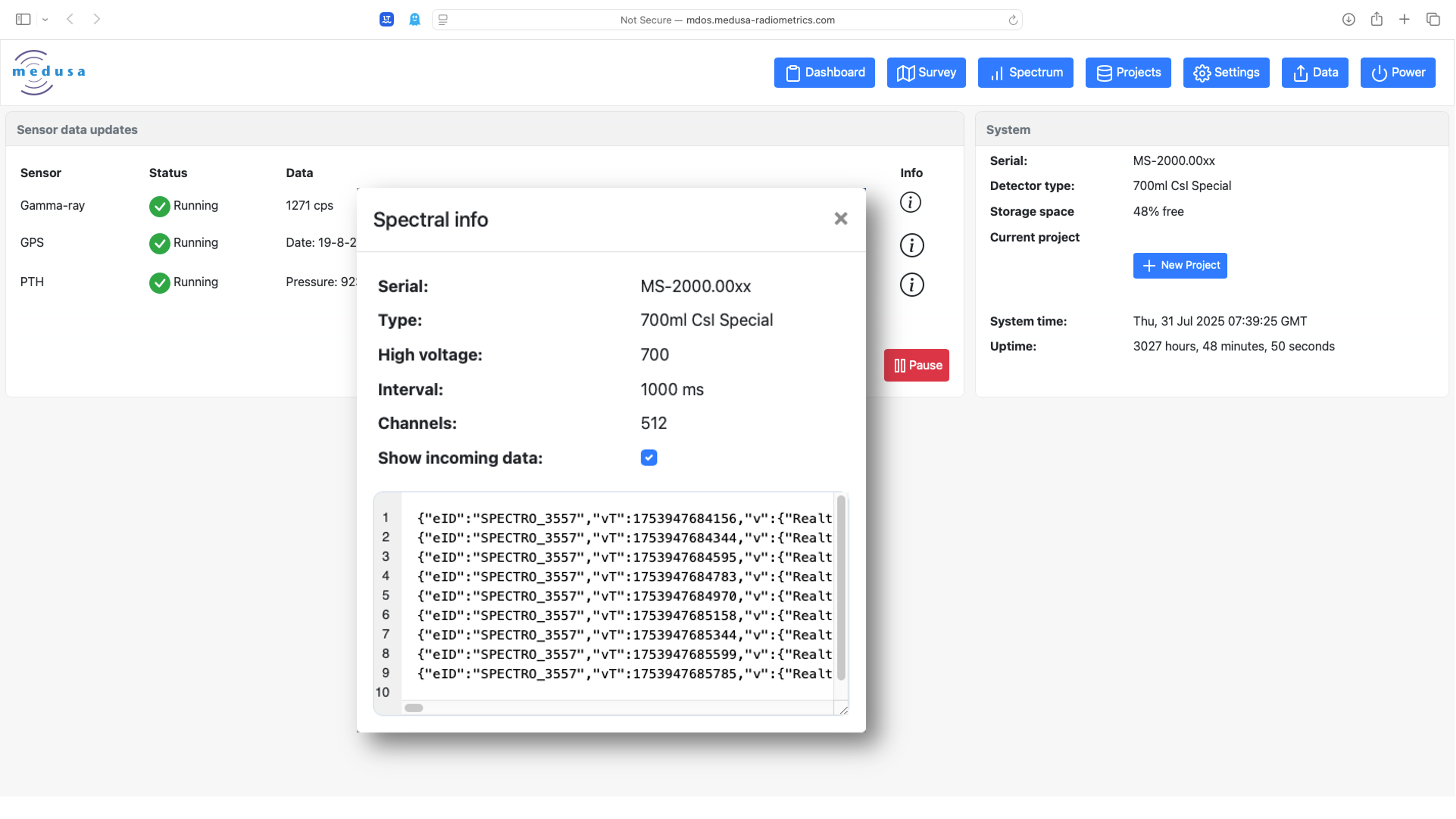
• When you get the interface, you will be at the “Dashboard” where you can see the status of the all sensors (gamma-ray, GPS, and PTH [pressure, temperature and humidity for post-processing]) on the detector. All of them should have a green tick.

• You can further inspect the data coming in by pressing the button on the right side of the sensor line.

Starting a survey

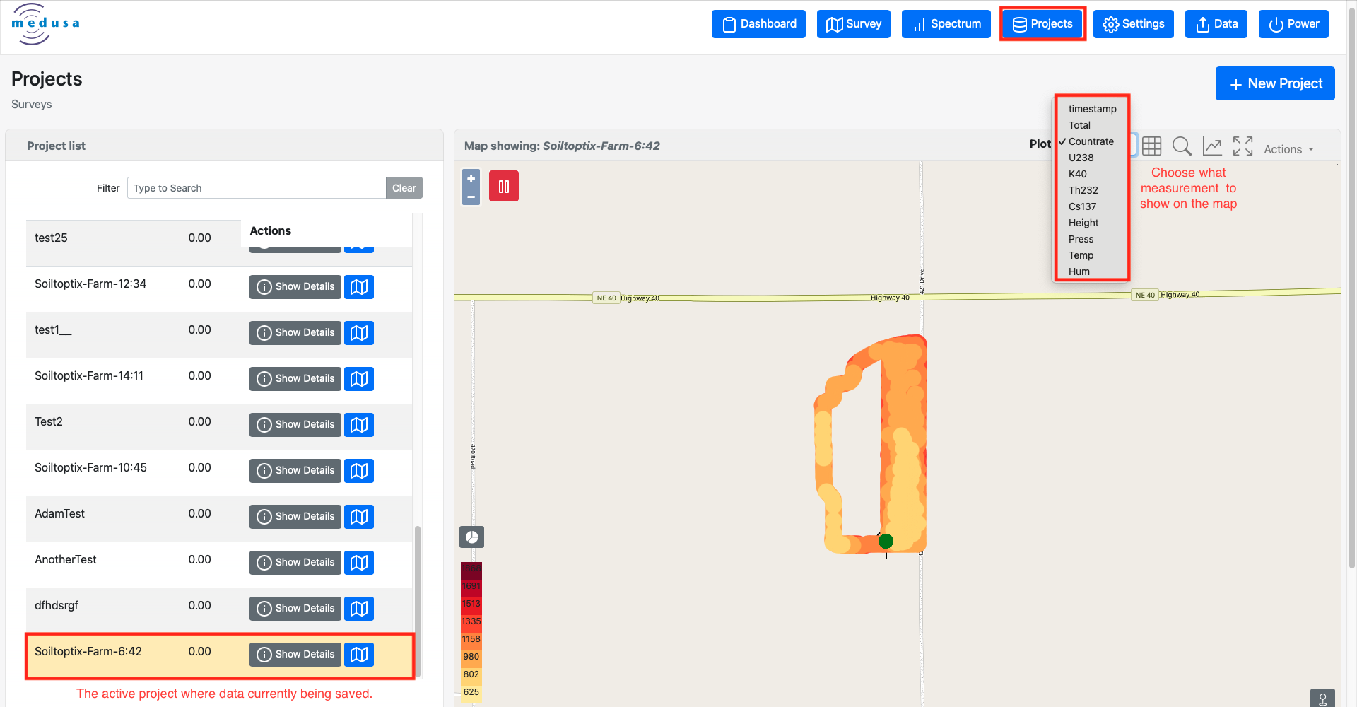
• You can create a project in dashboard or by going to the “Project” page from the blue menu. Please remember that your measurements are saved in the yellow highlighted project in the project list.

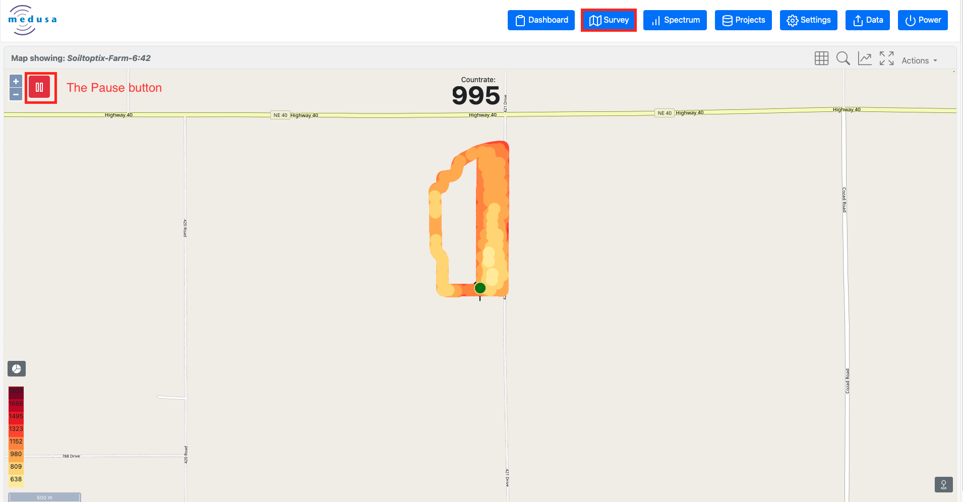
• The “Survey” page shows your position, adds data to the map as you measure. The color range indicates the range of mean ± 1σ and mean ± 2σ.

• Detector measures continuously as long as it has power. If you want to pause the sensor while moving between measurement areas (can be on foot surveys) with a vehicle or for any other reason (lunch break etc.), the red [II] button at the top left pauses the measurement, and the pause button turns into a green [>] resume button. The data collected during the pauses will be excluded from your data and can be reached later if necessary.

• During the survey, you can follow the measurement grid from the map at the survey page.

You can download an Open Street Map basemap. However, for this the sensor needs to be connected to the internet, which is possible only with an Ethernet cable.

• Keep an eye on the data coming in while on the survey tab. You should see the countrate and position change while moving. On the “projects” page you can select the total count, or individual ⁴⁰K, ²³⁸U or ²³²Th concentrations. Also, you can see the incoming spectra from the “Spectrum” page.

After the survey

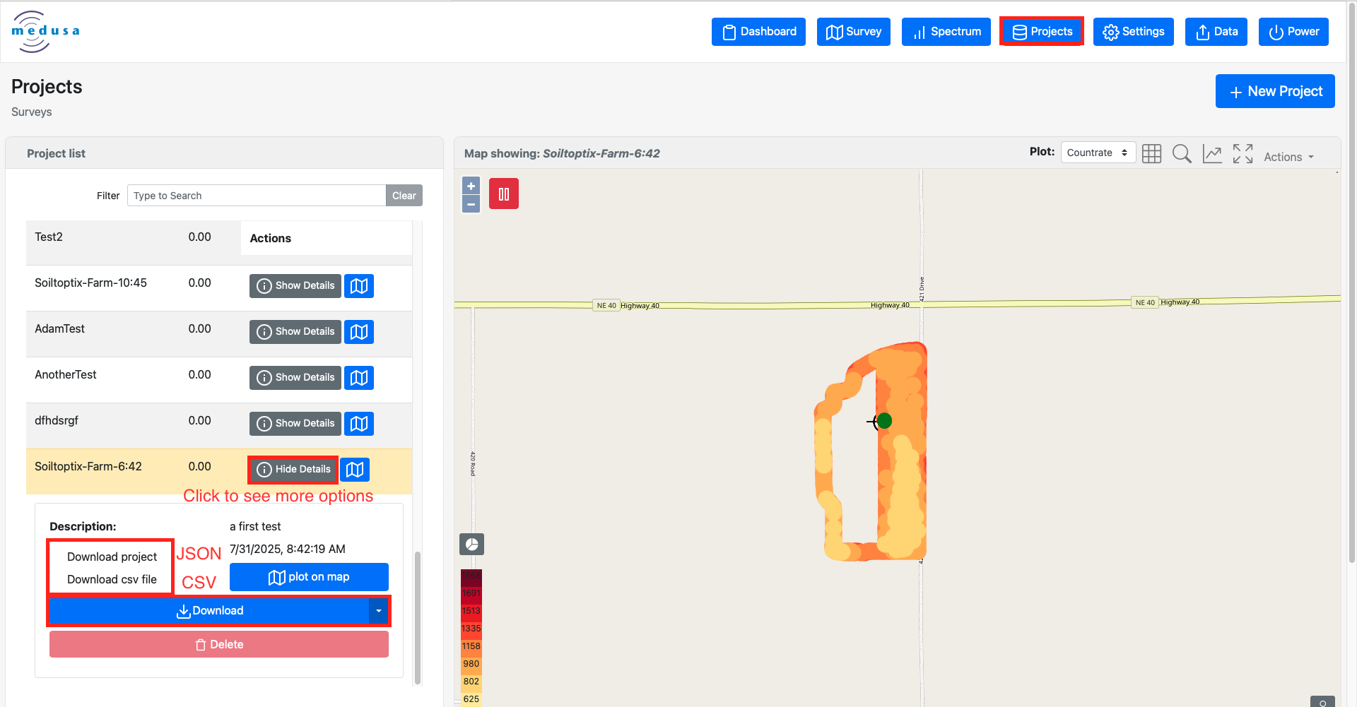
• To download the measurement data, go to the “Projects”, and click on the project you are interested. By clicking (info) icon, you can see more options for that project, and download the data by tapping on the blue download button.

• Two download options appear on the left: “Download Project” and “Download CSV”. For a quick look check of data from a survey in progress, click the second, “Download CSV”. This will send a short CSV file containing the georeferenced radionuclide concentrations and PTH data. Load this into any suitable data visualisation software, such as Geosoft or QGIS.

If the detector is configured with the right data-analysis settings and no special corrections need to be applied such as height corrections. This CSV can be used directly and the post-processing step can be omitted.

• Radionuclide concentrations are given in Bq/kg, but this can be changed to percentage for ⁴⁰K, and ppm for ²³⁸U and ²³²Th on the settings page. Cesium is always presented in Bq/kg.

• “Download Project” gives you an mDOS JSON file containing all data, including spectra for each reading. The JSON files have the name format: YYYYMMDDTHHMMSS<project name>.json, where the date and time are GPS-derived UTC values.

• From the main blue menu bar, you can reach the “Settings” page. Besides adjusting the sample

  rate and other parameters (Do not change these for normal surveys. These are for advance users.), you can see internal memory condition. If the sensor’s internal memory is getting full, you can do some housekeeping. Make sure all projects have been fully downloaded and backed up before deleting any!

Shutting down

• At the end of the day, just disconnect the power cable to stop the measurement.

• Remove the GPS antenna and the power cable and put everything back in the box for transport.

Post processing analysis

Importing data into Gamman

• The analyzing and visualizing the data in JSON file can be done using GAMMAN. The GAMMAN manual is available at https://docs.medusa-radiometrics.com/gamman-manual/latest/.

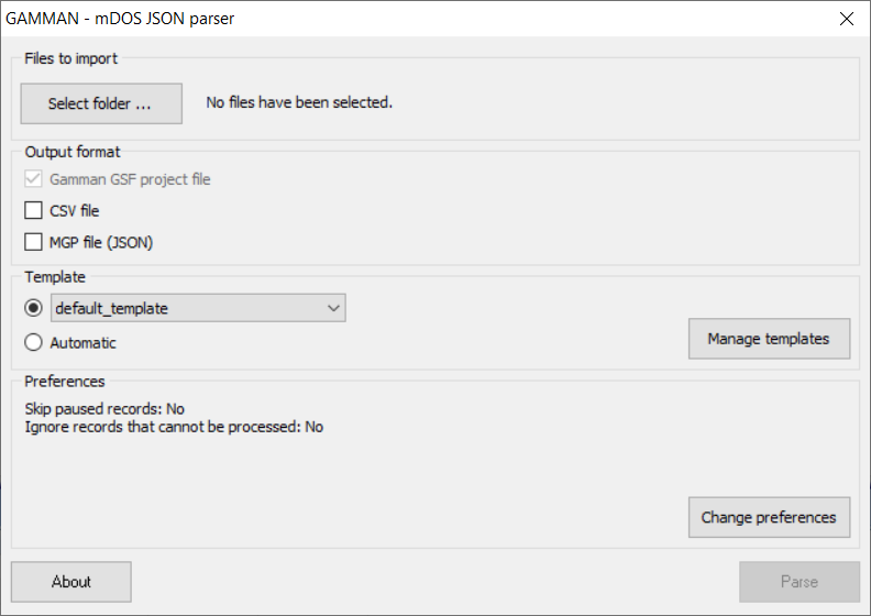
• Open GAMMAN and go to File/Create from/mDOS JSON files, or click “Create from mDOS json” button on the menu bar to open “mDOS JSON parser”.

• Select a folder that includes the JSON file(s), specify a template (or create one), check (or uncheck) the ‘Skip “paused” records’ box in Preferences and hit the ‘Parse’ button.

• You can choose which data items to display (spectra, GPS and PTH), and the order in which they appear. You can save the way you import the data in this screen as a template.

• Click OK and the JSON will load. This may take a while depending on the size of your JSON file.

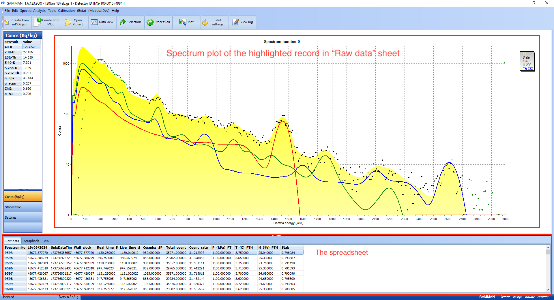
• Once the JSON is upload, a spectrum plot appears above, with the numeric data in a spreadsheet format below.

Visualizing and cleaning data

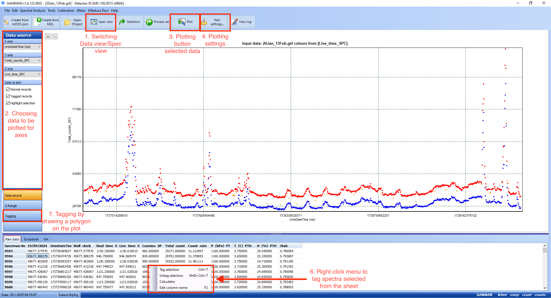
• GAMMAN can visualize any three columns from this table in a scatter plot: one in x-axis, one in y-axis, and the last one as dots with scaled colors.

• From the buttons on the top, click the “Spec view” / “Data view” to toggle between them. For a map plot, while in “Data view”, click “Data Source” and select X_GPS for x-axis, Y_GPS for y-axis and the data item you want to inspect with color map for z-axis, then click the “Plot” button.

• If your data is not plotted properly, you may need to check GPS data scrolling up and down on the data table. You have probably some null or incorrect GPS data. If this is the case, select and delete those rows. Also, you may check the “Plot settings” button, then “Chart/Axis/Left axis/Scales” and ensure that the “Automatic” box is ticked, and repeat this for “Bottom axis”.

• Unwanted data points can be tagged in the raw or processed data for deletion, exclusion from plots, or flagging as special interest in “Data view” —either directly in the data table or by drawing a polygon around them on the plot.

• In the data table, select rows (drag mouse holding left click or use CTRL + A to select all items), right-click to choose “Tag selection” (tagged rows are marked red); to undo, reselect and choose “Clear selection” or use options under the Edit menu like “Clear all tags.”

• On the plot, clicking a data point highlights its corresponding row in the data table—useful for tagging individual points or identifying the start and end of a group to be tagged.

• To tag points geographically, select Tagging from the sidebar, then hold Alt key and click to draw a polygon around unwanted points; close the shape by clicking the first vertex and press “Tag records”. To tag points outside a boundary, tag the inside points first, then choose “Invert tagged” from the Edit menu.

• To delete tagged points, use “Delete tagged” from the Edit menu. Alternatively, trimming to boundaries can be postponed until after importing the processed data into GIS.

Optional: restabilizing data

Stabilizing spectra is converting the raw spectrum data to a spectrum on an energy scale: a crucial process for radionuclide analysis.

• The stabilization of spectra is done by Gamman during import process. This can be improved using the “Stabilization editor” in Gamman.

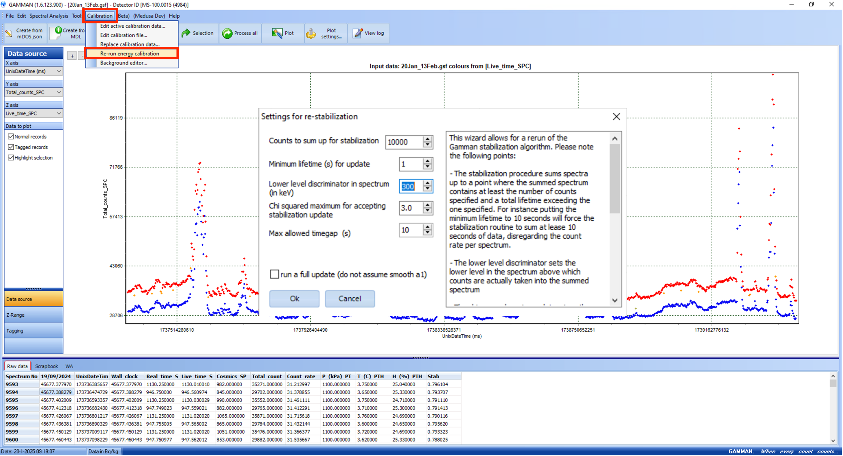
• After tagging and deleting unwanted data points, such as spikes or distortions, run “Calibration/Re-run energy calibration” to address any stabilization issues.

• When the stabilization dialog appears, the settings in this dialog box are important for a proper stabilization and should be suitable for an average user (avoid using the mouse scroll wheel, as it may unintentionally alter highlighted parameters). If manual adjustments are still needed, refer to the documentation.

• Stabilized spectra are used to calculate the nuclide concentrations.

Data analysis

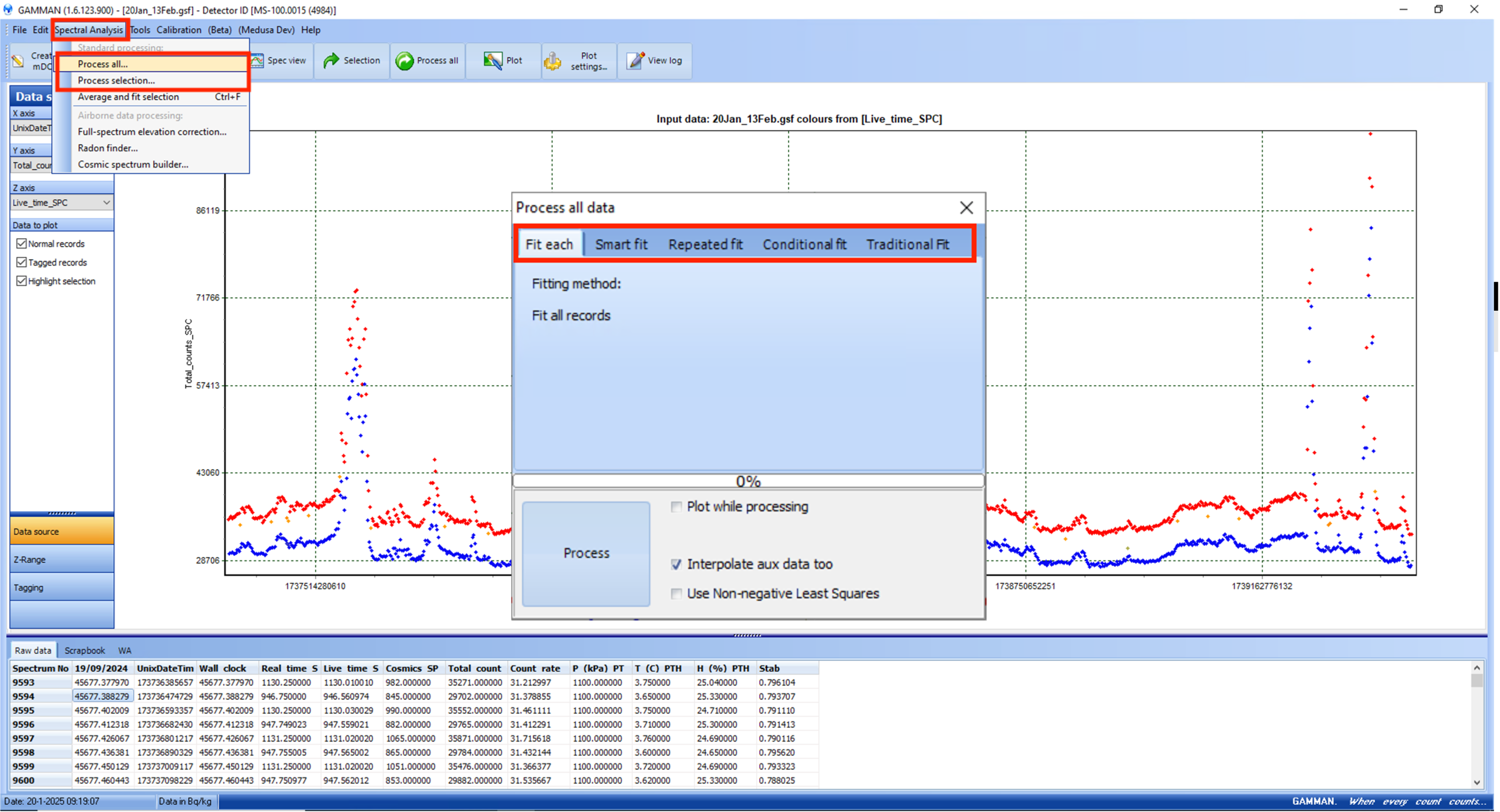
On the menu bar, “Spectral Analysis/Process all (or selection) brings you to a menu with several calculation methods. Detailed information on these methods can be found in the Gamman manual and a short description is given in the table below.

• Ticking “Plot while processing” can be make the process slower. By ticking the box “Use Non-negative Least Squares”, you can avoid getting negative concentration values.

• If you are not an advanced user, Repeated fit is a good to go method.

The advise it to start with a repeated fit of 5 and look at the uncertainties in the resulting concentrations. If they are good you can reduce it to a repeated fit of 3, if they should be improved you can use a repeated fit of 7.

Note that by increasing the number of records summed you improve the point uncertainty, but at the cost of your spatial uncertainty, because more points are averaged. The goal is to find an acceptable point uncertainty with the minimal number of records summed.

Exporting data

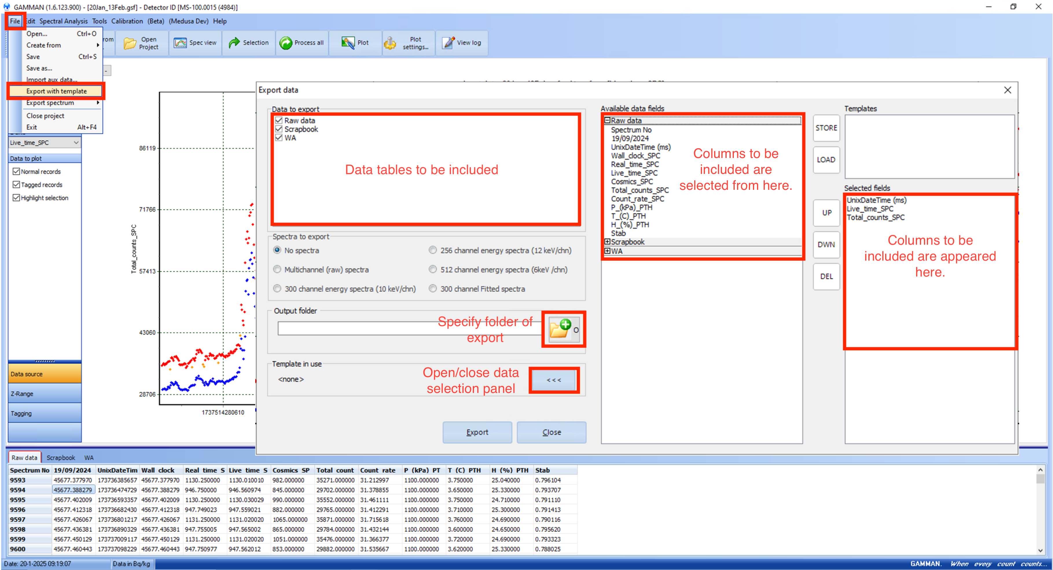
• After processing, export results via “File/Export with template” to a CSV file. You can choose what to include in the file from “Data to export” —the raw and/or processed data. “Spectra to export” is for inclusion of spectra. The button “>>>” in the area “Template in use” opens a menu with three fields. From “Available data fields” you can choose what to include column by column, by double-clicking on each. “Selected fields” shows the included columns. Finally, hitting the “Export” button will create the CSV file in the folder indicated in “Output folder” by asking you the file name at the last step.

• Each data process attempts (with different methods or on different sub part of the raw data) will create another data table next to “Raw data” tab, and each will have the same column name. Therefore, it is a good practice to import each data table to different files to avoid confusion.

Questions or Support

For technical support or questions about this manual, please contact Medusa Radiometrics at support@medusa-radiometrics.com or consult the latest documentation at https://docs.medusa-radiometrics.com .