A GR820 test at the Breckenridge

The data below is taken with a (4x4x16inch NaI-based) GR820 system. The system was used in a comparison test with a Medusa MS-4000 spectrometer. The set is shared here as an example of 3rd party data and how to use that inside Gamman.

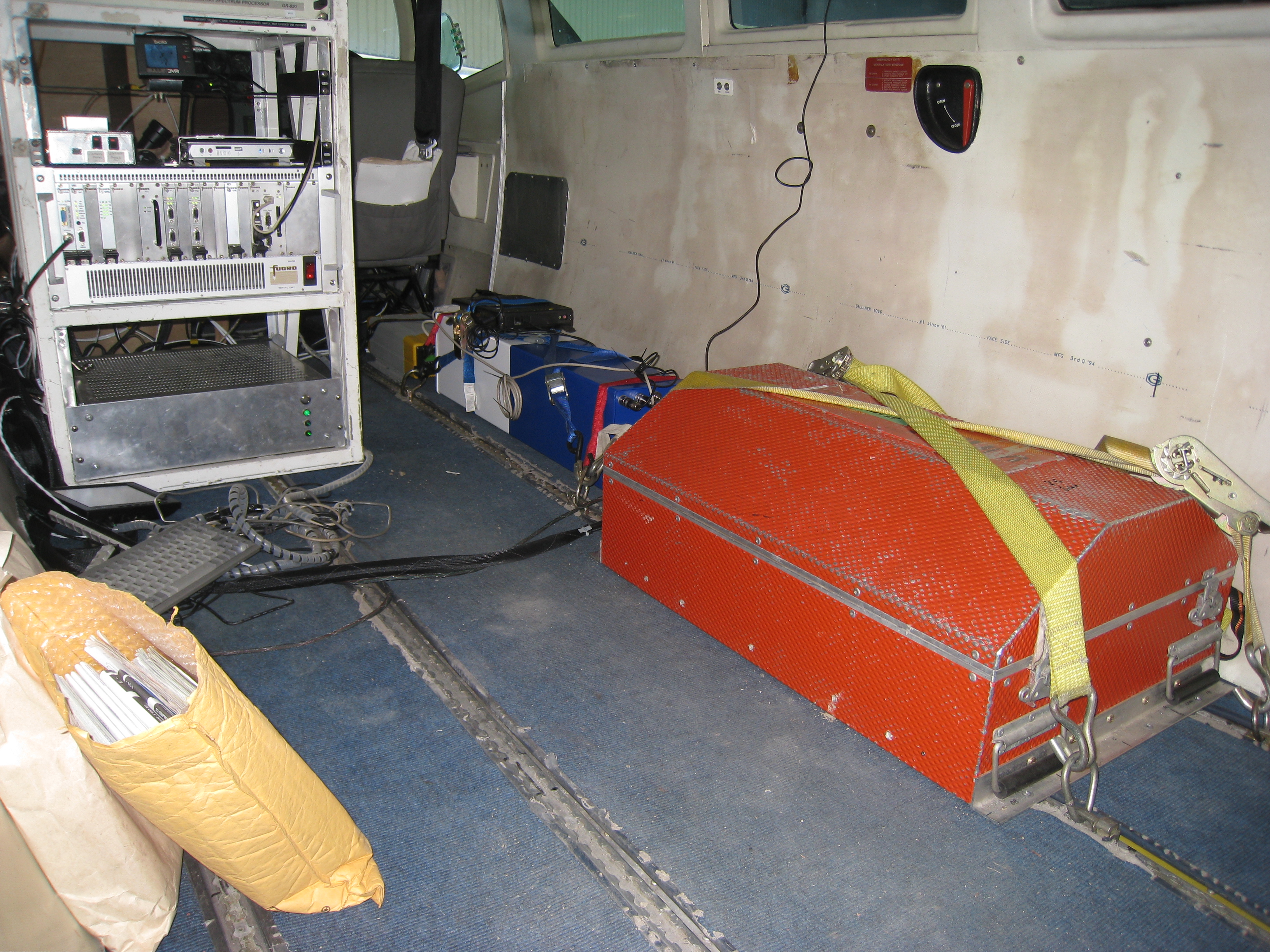
Front: the red GR820 box containing 5 4x4x16 NaI crystals. Back: the Medusa MS-4000 CsI based system. Platform: Cessna 404 Titan (Fugro Airborne Services 2010)

Survey purpose	Test on Breckenridge range
Gamma-ray system	GR-820 (5 x 4L naI
Survey platform	Cessna 404 Titan
Data provider	Fugro Airborne Surveys, Ottawa (CA)
Dataset	The XYZ file exported from a Geosoft Database file; The GSF that was created using this XYZ file A calibration file (MCF) for the GR820 F DOC describing the channels.
Notes	The Fugro dataset contains 2 256-channel spectra per row. The first spectrum is the summed spectrum of the 4 downward-looking detectors; the 2nd is the upward-looking detector. Current Gamman does not support reading both spectra into a single project file. To use both spectra one should create 2 separate Gamman projects. The upward looking detector set could then be used to extract radon or cosmic count rates.
Download	GR820 Fugro Breckenridge.zip

Step 1 - importing data

Below we show a few of the steps you’d need to take to get the Fugro data on-boarded in Gamman.

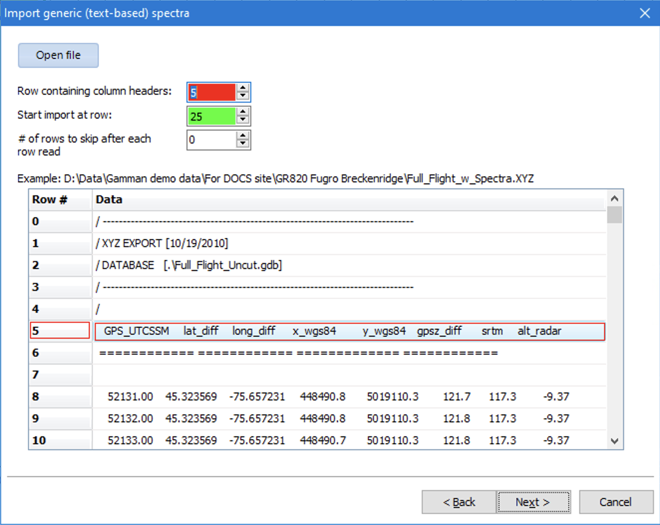
Step 1 - try to import the XYZ file. We start import at row 25 because some of the fields are empty (and marked “*”) in rows above. Gamman cannot read these “*” marks.

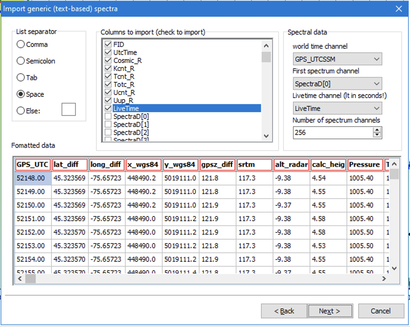
Step 2. The column separator is a space. Select all columns you want. Note the XYZ file contains the summed spectrum of thewnward looking and also on each row, the upward looking crystal. Gamman can only read one of these at the time.

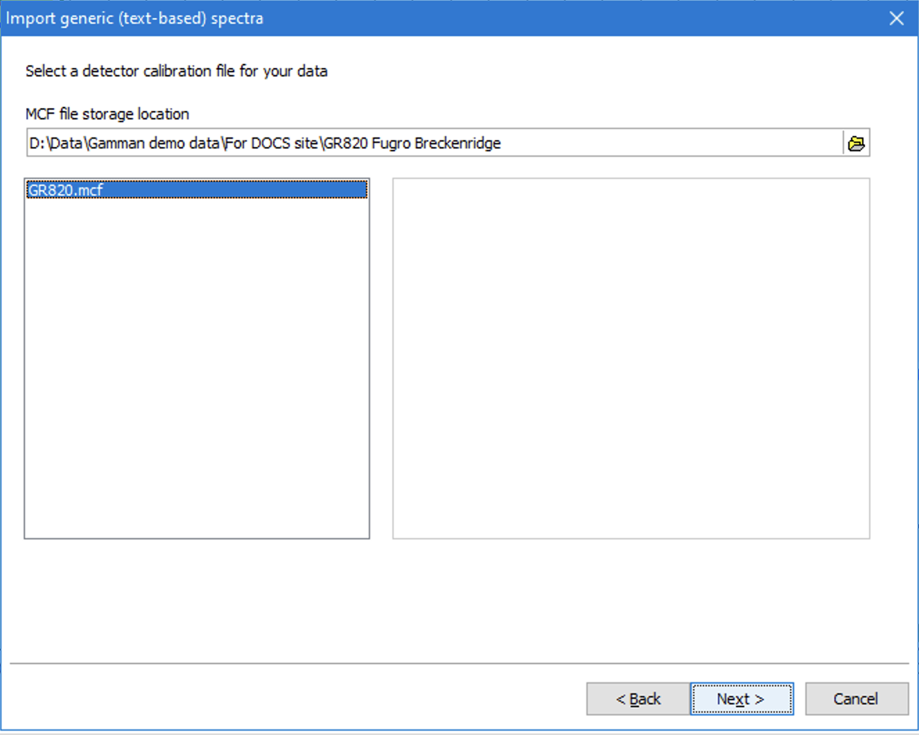
3rd step is to select a calibration file (that was made by Medusa for Fugro)

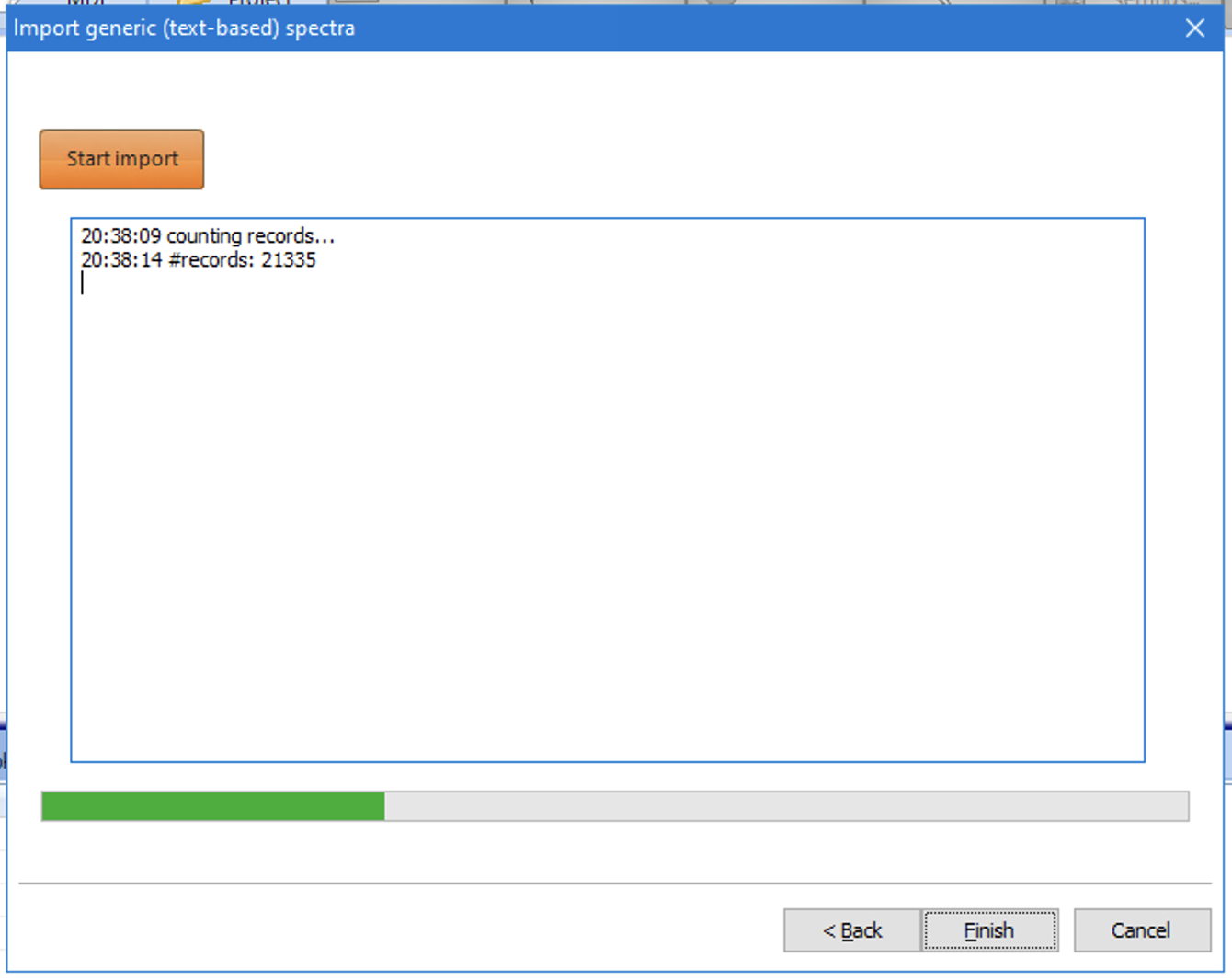
And then start importing the data (which can be a time-consuming operation)

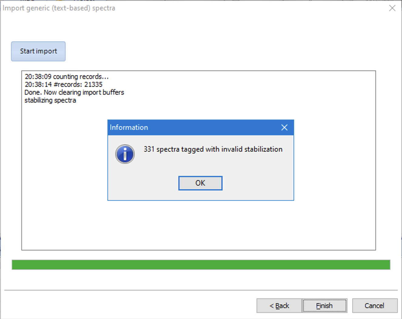
Last step is running a energy calibration check (“stabilization”) on all imported spectra. You might get this popup telling you there are some suspicious spectra in your dataset. You can easily find them by plotting tagged records only.

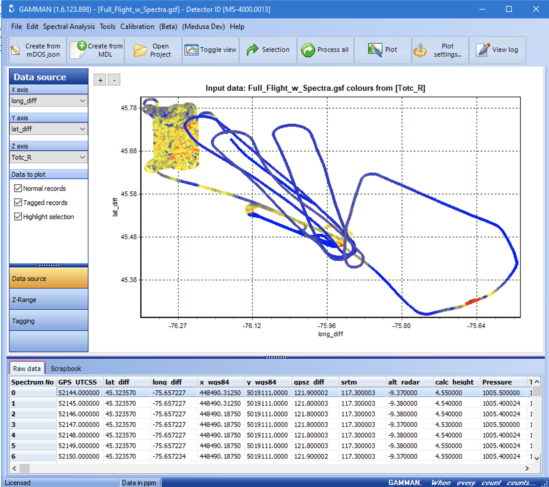
And finally you will end up with a picture like this - a plot (in this case) of the area flown with colors mapped from the Tote_R column.

Step 2: extracting cosmic and carrier backgrounds.

This dataset has a nice piece of data flown at very high altitudes. This allows to extract the cosmic spectrum that subsequently can be used as a background to the rest of the data.

Gamman supports 2 modi for retrieving cosmic and plane backgrounds.

Method 1 - “classic” extraction using cosmic channel scaling

Method info: check https://docs.medusa-radiometrics.com/gamman-manual/latest/9-cosmic-and-carrier-backgrounds

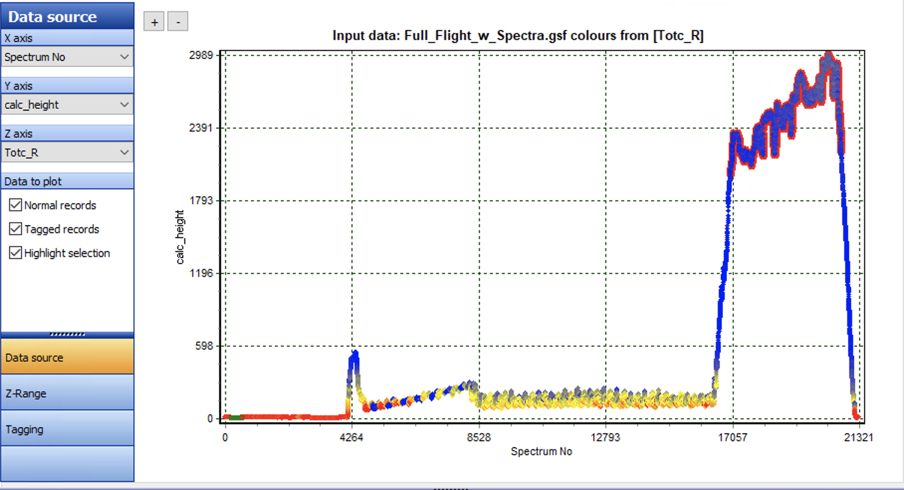
First plot the calculated height as a function of spectrum no. Then select the high-flown part (the part between record 17000 and 20000).

Now open the “classic” background finder: [menu.tools.classic cosmic background]:

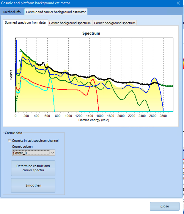
Make sure to select the output column containing the cosmic counts. Then run the “Determine…” knob. After a while you will see the image below:

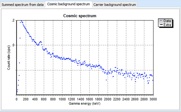
You can now choose to smoothen the cosmic spectrum and save it for further processing.

FSA-version

An alternative method is based on full spectrum analysis. In this method, Gamman fits a cosmic background spectrum to the spectrum measured at height. The cosmic spectrum is modelled using MCNP assuming a number of known atmospheric gamma lines that arise from incoming high-energy cosmic radiation.

The advantage of using the FSA version is that there is no need to fly steady for 15-30 minutes at a number of different high altitudes. The only requirement is fly high enough to avoid radiation from the soil in the spectrum - best would be to fly high above sea.

First - again - select a certain high-flown range and open [menu.spectral analysis.cosmic spectrum builder}:

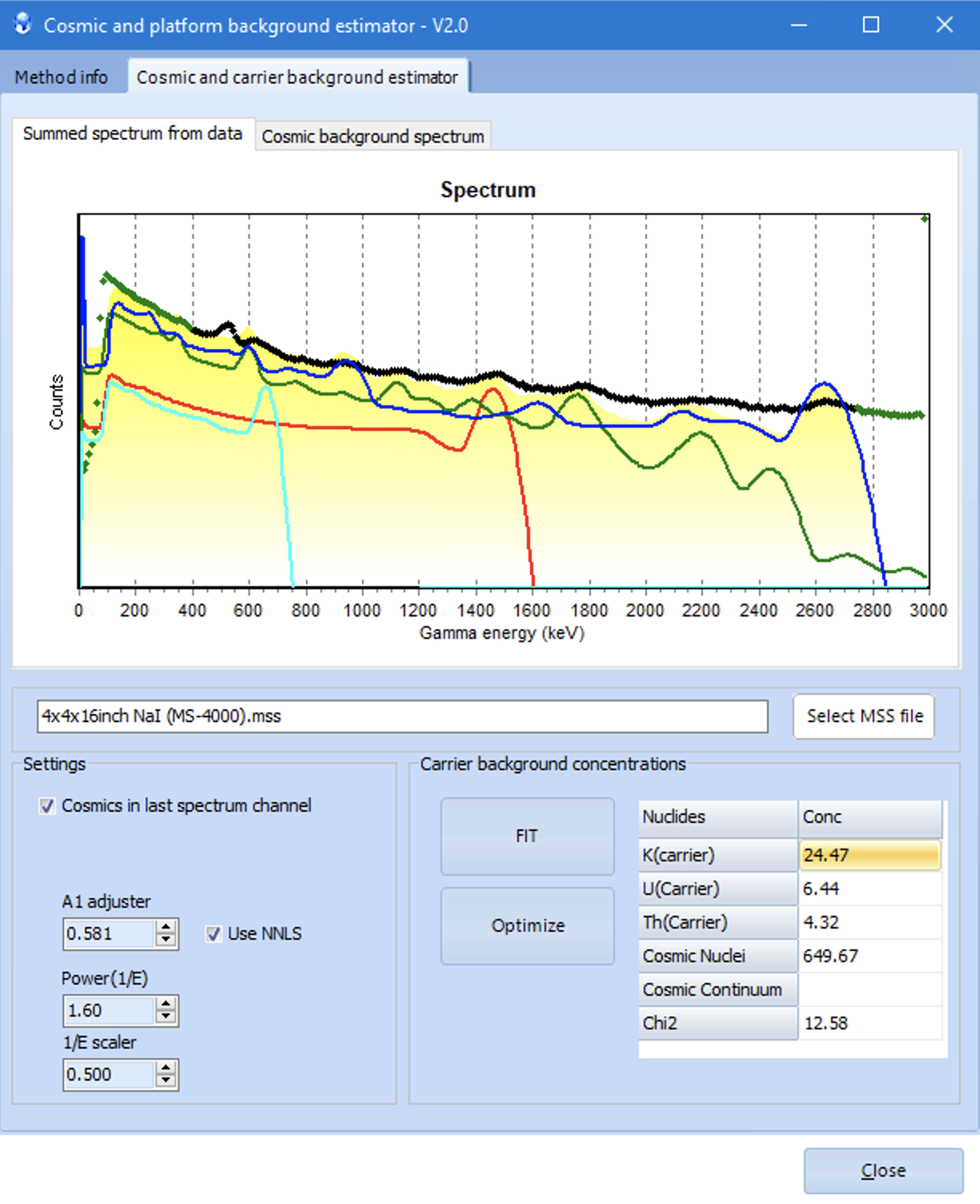
Then open the “Cosmic Spectrum Builder” under the Spectral Analysis menu. Make sure to select the 4x4x16 NaI MSS file. The spectrum shown above is the summed spectrum over the range selected in the previous picture

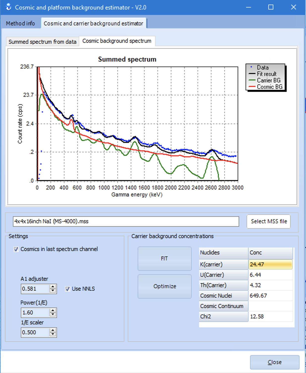
Select the Cost Background Spectrum tab - and play around with the settings. For more info on the method(s) see https://docs.medusa-radiometrics.com/gamman-manual/latest/1-cosmic-background-spectra-in-gamman. Close the wizard to save the cosmic background to your GSF file.

Step 3 - radon corrections.

We omit this step here as in the data there is no clear Radon signature.

Step 4: elevation corrections

The last step would be to run elevation corrections on your data. There are (again) 2 ways to proceed:

Full spectrum airborne corrections. See https://docs.medusa-radiometrics.com/gamman-manual/latest/11-the-airborne-corrections-wizard
“Classic” airborne corrections.