Sample suggestion algorithm

The goal of sampling is to find relationships between radio nuclide measurements and soil properties that can be measured only in the lab. This way, it is possible to use gamma-ray spectrometry to measure properties of interest indirectly, using field measurements as a proxy.

The sample suggestion algorithm tries to identify sample locations that have an optimum in both spatial and count rate distribution. The number of samples is based on the calculated area size and by a predefined sample density in samples per ha.

Raw survey data

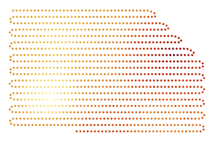
The figure below shows an example field with measurements collected by driving/flying back and forth to cover a complete area of interest. Each dot in the image describes a single collected spectrum, colored by count rate.

Dividing the mapped area into squares

The algorithm will first determine the boundaries of the mapped field. In this process, any outliers such as dots with poor GPS coverage are removed from the data set.

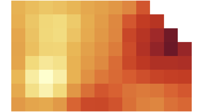
The surveyed area is divided into equal sized squares, where each square's center is a potential sample location. The number of squares, and therefore the number of potential sample locations depends on the total number of measurements and the space between measurement lines. The figure below shows the same field as before, but divided in squares.

Info

The sample algorithm can work with separate areas, where the squares do not form a single area, but it works best for simple fields that form one contiguous area.

Grouping squares into count-rate sections

Squares are sorted by count rate and grouped into as many sections as there are samples to place, one section per sample. Assuming a normal distribution, all but two of the sections evenly split -2 to +2 standard deviations; the remaining two outer sections cover everything beyond that range. Since the outer sections are naturally thin, each is expanded to at least three squares. The figure below shows the squares, sorted by count rate. Black lines mark the section boundaries.

Selecting the sample locations

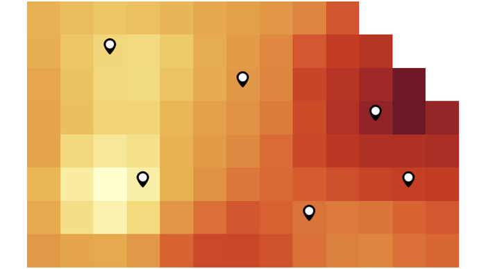
One square is picked from each section, so the samples span the full count-rate range. Within each section, the algorithm picks a square so that the combination gives the best-spread overall set. A location's score is its distance to the nearest other sample and to the field boundary, with the boundary distance counted at a fixed 1:2 ratio: a sample only needs to be half as far from the edge as from its nearest neighbor to score equally well. This keeps samples out of corners and pushes them toward sitting twice as far from each other as from the edge. Forcing one sample per section deliberately biases the selection toward some unusually high and low readings. A relationship between field and lab measurements is far more reliable when the samples span the widest possible range, not just the average.

Optional: soil texture samples

Analyzing samples for soil texture is expensive, so the algorithm can suggest a smaller subset of samples for soil texture analysis. This option is enabled by checking the "Include texture advice" setting before running the sample suggestion algorithm. The soil texture subset is chosen with the same algorithm, but the only candidates are the sample locations themselves. The number of soil-texture samples depends on the number of samples in the original set.

Summary

The algorithm discards positioning errors and unreliable squares, grids the field into average count rates, groups squares by count rate, and picks one sample per group - spread across the field, away from the boundary, and spanning the widest range of count rates. The number of samples itself is not fixed: it is based on the calculated area size and a predefined sample density. An optional smaller texture subset can be drawn from those same locations.